Lab 2: Introduction to R and RStudio
Introduction
This lab is designed to introduce you to R and RStudio, which we will use for all future computer labs. R is a high-level scientific scripting (programming) language for analyzing and visualizing data. RStudio provides a useful front-end visual interface for writing R code and viewing results. “High-level” here means that the grammar of the R programming language is designed to be reasonably intuitive to humans, as opposed to other programming languages that are optimized to be machine-readable. R is part of a whole family of high-level programming languages – Python and Matlab are also very popular, plus ArcGIS, JavaScript, etc., etc. When learning any of these languages, the rule of thumb is that the first one takes the most time to learn, but after that, the next one is relatively easy to learn, because they all follow similar conventions. Knowing one or more of these languages is a foundational skill in the fast-growing field of the data sciences.
Before the lab
Download R and RStudio and familiarise yourself with the layout.
RStudio is an integrated development environment (IDE) for R and runs R under the hood (you will need both installed). There are other options available but we will stick with RStudio.
Getting help in Geog523
R is hard, we know, and we can’t teach it all in one lab. Take advantage of the out-of-class resources including the slack channel and office-hours. We are here to support you through the learning curve. While coursework should be completed independently we also encourage students to help each other out.
This workbook is intended to provide you with some basics skills, but primarily to direct you to relevant resources. Links will be provided along the way and in Section 6 are resources (some of which this lab is based on) that include everything needed for this module.
When posting in the Geog523 slack channel:
Make sure you have looked through the resources and tried to solve the problem yourself.
Ask a clear question copying the line of code causing an error as well as the error message.
Best practice for asking questions is to create a ‘reprex’. Often you will solve your own question by working it through.
R basics
Buckle up, here we go! We will have regular check-ins during the lab to make sure everyone is keeping up.
Why use R?
Coding is an essential skill to any data-science and analysis. Software such as R is:
reproducible (unlike point and click software)
capable complicated analyses
open source
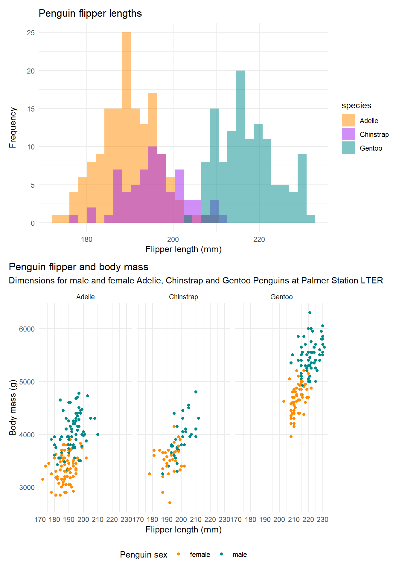
Data visualisation is an important part of communicating results. Below is an example of visualisations of penguin morphometric data. We will be visualising palaeoecological data later in the course.
RStudio interface
RStudio has four main panels (the source panel will appear after you open an R script):
Source is where your script displays.
Environment where data, objects and functions are shown.
Console where the code runs (either from your script or written directly into the console).
Files, plots… Where you can view your files, plots package help and plots.
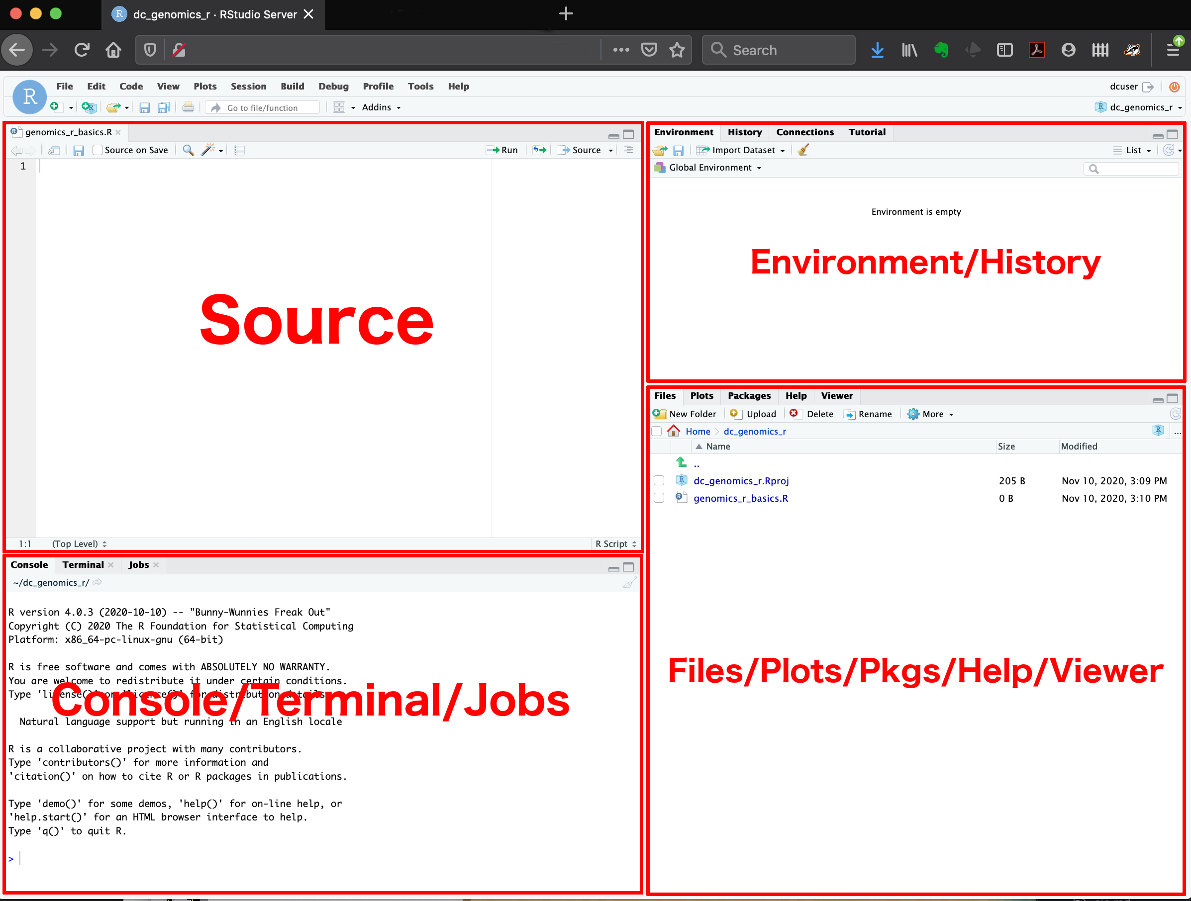
Each panel has multiple tabs for different features, for example there is a ‘Terminal’ tab next to the ‘Console’ tab for operating the terminal rather than R.
Projects and Working Directories
It is important to structure projects carefully from the outset so that data and scripts are stored in the same location. Usually a project’s structure will have a high level directory that contains several sub-directories for data and outputs. For example you might want to create a course directory called ‘2022-Geog523’, a directory within that for this lab called ‘02-intro-to-r’, and two sub-directories within that named ‘data’ and ‘outputs’ respectively that we will use later.
Reference resource
- 2022-Geog523
- 02-intro-to-r
- data
- outputs
- 02-intro-to-r
Future labs will be set up following a similar structure.
Exercise
Create the described directory structure above
Open up RStudio click ‘File’ -> ‘New Project’ -> ‘Existing Directory’. Navigate to the directory you created called 02-intro-to-r and hit Create Project.
Create an R script (Click ‘file’ -> ‘New File’ -> ‘R Script’)
Math operators
Fundamentally, R does math. In other words, R supports mathematical operators:
2 + 3[1] 5(2 + 3) * 7[1] 35pi / 4 # note that 'pi' is built into R.[1] 0.7853982
Exercise
Write the calculation
pi * 3^2in your R script and hitctr + enterto run it in the console.Save your R script to the high level directory you created earlier called 02-intro-to-r.
Objects and assignment
Typically we work with ‘objects’ in R. An object can be a value, word, data, matrix, or any acceptable type in R (more on types later). Objects are displyed in the ‘environment’ (by default, the top right panel) in RStudio. To create an object we use the ‘assignment’ operaror (<-).
Reference resource
# Assign a value of 3 to an object called 'radius'.
radius <- 3
# See it appear in your 'working environment'?

# Assign a value to an object called 'area'.
area <- pi * radius^2
# the assigned value is the result of the calculation on the right hand side of the assignment operator (<-).
These lines of code first, assign a value of 3 to an object called ‘radius’ and then assign the result of a calculation (using the object radius) to a second object called ‘area’. pi is predefined in R; thus, does not need to be assigned to an object.
Note that assignment does not print the result. To do so we can ‘call’ the object by running it (control enter).
# By running the name of an object it will 'print' the output to the console.
radius
[1] 3area[1] 28.27433
Exercise
The formula for the volume of a sphere is: \(\frac{4}{3}\pi r^3\)
assign a value to an object
raduisassign the output of the calculation for the volume of a sphere to an object called
sphere_volume
Note object names cannot have spaces or begin with numbers. Use snake_case or CamelCase
Functions and help
There are many functions built into R to make life easier. Functions are easy to recognise because most are a function name followed by parentheses, e.g., sqrt(). Requirements of the function are put inside the parentheses and are called ‘arguments’. A function takes an input (or several) and produces an output. For example:
# Take the square root of the number 16.
sqrt(16) # '16' is the input provided to the function sqrt.
[1] 4sqrt(radius) # Take the square root of the object defined earlier.[1] 1.732051round(area) # Round up the result of area.[1] 28
Reference resource
Using functions for more detail.
Note that we are performing calculations on the object but not overwriting it. The objects radius and area still retain their original values. We could overwrite the object like this:
radius <- sqrt(radius) # run the object radius again to see the new value.
# or create a new one like this:
area_round <- round(area)
Functions can be simple (like the examples above), or designed to complete sophisticated analyses. To find out more about a function you can bring up the help using the ? followed by the function name:
?roundSee the help for the function round tells you the details? If you scroll down to the ‘Arguments’ section you will see it has a second argument called digits. You will also see examples of how to use the function.
Exercise
- See if you can use the
round()function and thedigitsargument to round theradiusobject to different numbers of decimal places.
Packages
R has a set of functions built in like the examples above but often we need more that come from downloading packages. A package is a collection of functions. Packages are often specialized to complete particular tasks and analyses. A lot of learning R is figuring out the functions you need.
To install a package we use the function install.packages() and put the name of the package in quotation marks:
install.packages("palmerpenguins")
install.packages("ggplot2")
To access the set of functions in a package we have to tell R to load them using the library() function:
library(palmerpenguins)
library(ggplot2)
Now R knows we want to access functions from the palmerpenguins package. More on this later in the course.
Data types and structures
Data types and structures are important concepts in R. The objects we worked with, radius and area, were both type double (decimal). Other types include: characters (also called strings), integers, logical, and factor.
Reference resource
char <- "this is a string" # A string is indicated by ""
int <- 42L # Integers are indicated by the 'L'
doub <- 1.61803 # Double (can also be single digits)
logic <- TRUE # Logical types are TRUE or FALSE (case sensitie)
fact <- factor(c("small", "medium", "large", "large")) # factors or categories
To find the type of an object use the function class(). The radius and area objects are vector objects of length 1. Other structures exists such as lists and arrays which we will leave alone for now. The function c() used above concatenates (sticks together) multiple values that must be of the same type into a vector.
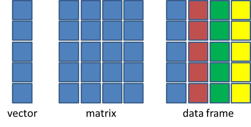
Data structures are organised sets of values. The most fundamental are:
Vectors: one dimensional structures of a single type
Matrices: two dimensional structures of a single type
Data frames: two dimensional structures of mixed types
Vector examples
# Create a vector of type double
doub_vec <- c(1.87, 5, 42, 10.0)
# Create a factor vector, a special type of vector indicating categories.
factor_vec <- factor(c("small", "medium", "large", "large"))
int_vec <- c(1L, 2L, 3L, 4L) # 'L' indicates an integer.
Matrix example
The matrix() function creates a two dimensional matrix that must also be of the same type.
# creats a 5x2 matrix from the numbers 1 to 10
A <- matrix(1:10, nrow = 5, ncol = 2) # the ':' means 'to', e.g., from 1 to 10.
A
[,1] [,2]
[1,] 1 6
[2,] 2 7
[3,] 3 8
[4,] 4 9
[5,] 5 10Data frame examples
A data frame can store data of mixed types. That is, each column can have a different type, you may have a column of strings (e.g., species names), and a column of values belonging to each species (e.g., abundances). The data.frame() function can combine the vectors into a data frame.
data_mixed <- data.frame(factor_vec, doub_vec, int_vec)
data_mixed
factor_vec doub_vec int_vec
1 small 1.87 1
2 medium 5.00 2
3 large 42.00 3
4 large 10.00 4
Exercise
- use the functions
class(),str(),dim(), andcolnames()on the objectdata_mixed- use the help
?to find out what the functions do
- use the help
Saving and loading data
Let’s now save the data frame we created to our data directory. The base R functions for saving and loading data as a .csv file are write.csv() and read.csv().
The write.csv() function requires arguments of: the object you want to save; and where you want to save it. If you forget, remember to look in the help ?write.csv.
# The first argument provided is the object we want to save
# The second argument 'path = ' has two parts:
# The directory to save the object to: 'data'
# The file name and extnesion: 'data_mixed.csv'
# note they are separated with a '/'
write.csv(data_mixed, file = "data/data_mixed.csv")
To load the data back into R we would use the read.csv() function. We will use this later in the course.
Plotting
To finish up with something fun, let’s check-out the penguins data shown at the start. The palmerpenguins package has a data frame called penguins built-in. The dataset describes morphological traits of three different species of penguin: Adelie, Chinstrap, and Gentoo Penguins. To load the data use:
data(package = 'palmerpenguins')
# Have a look at the data:
penguins
# What are the dimensions of the data:
dim(penguins)
The following code generates a plot of penguine body mass against flipper length and saves it to an object called mass_flipper. The three different species of penguin are plot using different shapes and colours. The plot is generated using the ggplot2 package. Have a look through the code and copy it to your script and run it. If you cannot make sense of the code at this point, don’t worry about it. We will be going through the details later in the course.
# Following example from: https://allisonhorst.github.io/palmerpenguins/articles/examples.html
mass_flipper <- ggplot(data = penguins,
                       aes(x = flipper_length_mm,
                           y = body_mass_g)) +
  geom_point(aes(color = species,
                 shape = species),
             size = 3,
             alpha = 0.8) +
  scale_color_manual(values = c("darkorange","purple","cyan4")) +
  labs(title = "Penguin size, Palmer Station LTER",
       subtitle = "Flipper length and body mass for Adelie, Chinstrap and Gentoo Penguins",
       x = "Flipper length (mm)",
       y = "Body mass (g)",
       color = "Penguin species",
       shape = "Penguin species") +
  theme(legend.position = c(0.2, 0.7),
        plot.title.position = "plot",
        plot.caption = element_text(hjust = 0, face= "italic"),
        plot.caption.position = "plot")

mass_flipper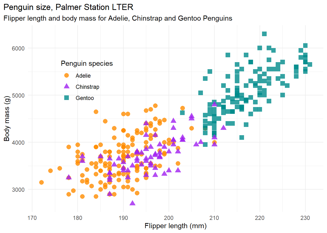
Now we can save the image to our outputs directory:
ggsave(filename = "outputs/mass_flipper.png", plot = mass_flipper, device = "png")Homework
As a starting point, if you are unfamiliar with R, go through this workbook again and link through to the reference resources provided along the way. Each link points to a useful recourse for each topic (assignment, objects, and data structures) that go into more detail.
Main Exercise
For the main exercise, we’re going to shamelessly borrow for this introductory lab exercise and have you work through the first three chapters of an on-line tutorial (PDF format) developed by W. J. Owen of the University of Richmond. You can obtain it here from CRAN and from our course lab folder on WiscBox
In WiscBox, there’s a starter script (i.e. R file) that you can use as a template for working through these exercises. During lab, Quinn and I are available as resources. I also strongly suggest that you look for ways to peer-mentor. Slack is an excellent avenue for posting questions to your classmates and instructors.
During lab, you’re free to work individually or in small groups of 2-3 people. OK also to work in groups outside of class. However, 1) I want each student to turn in their own assignment and 2) research shows that the student working at the computer learns much more than the student observing. So if you do work in pairs, be sure to regularly switch roles.
Once you’re done, please submit the R script to me via Canvas/Assignments. I’ll then review the code (and comments!) and test-run it.
Additional Comments on the Owen exercises
Overall
Be sure to comment your code! Good code is well-commented code. Usually the biggest beneficiary of well-commented code is the future you, so learn good habits early! In R, any line beginning with # is a comment line and the computer will skip it when running the code.
Section 1.2
You can skip this, and simply start RStudio. RStudio includes a window with a command-line interface for running R code.
Section 1.3
This command is already in the demo script – practice running it.
Section 1.4
Practice the ls() command. But note too that you can also look at the output in the Environment tab in upper right.
Section 1.5
Practice the help() command. But note that RStudio also provides a help option in the lower right window.
Section 1.7
You can skip this - but be sure to periodically save the scripts in your RStudio workspace.
Section 1.9
Q3: Don’t give me your phone number! How about your StudentID instead. Q4: An Identity Matrix is a square matrix (NRows=Ncolumns) in which all values in the principal diagonal (from upper left to lower right) are equal to 1, while every other value in the matrix is 0. Q5: Save the RStudio workspace and R script, rather than a txt file.
Section 3.4
Q3: No need to estimate your grade: just provide coursenumber and coursedays.
Resources
-
- In-depth resources, see: Hands-On Programming with R
-
- I recommend only browsing stackoverflow at this stage. The community does not like duplicated questions.
Tips and best practice
Here are additional tips to read in your own time that help make your scripting life easier. Some are general best practices that are useful to integrate while you learn how to code.
Layout and structure
R scripts can have a layout with headings that you can view by clicking the ‘outline’ symbol on the top right of your source panel. To insert a heading use either 5 hashtags: ##### Heading title or # Heading title --------------------------. Include plenty of comments. Writing informative comments is quite a skill.
# Libraries ---------------------------------------------------------------
# A list of required libraries and I like a comment indicating what they are for.
library() # For ...
source() # If you have any source functions (i.e., a separate script of functions you have written)

# Data wrangling ----------------------------------------------------------
# I like to set a file pathway with the 'here' package before reading in data
data_files <- read.csv()
The above code chunk is a good way to layout a script. Typically a list of libraries is included at the top (rather that dispersed throughout). Functions are sourced, then data are read in, manipulated, visualised and analysed.
Comments
When writing code it is best practice to include comments. When you look back at your code in a week or two it can be difficult to understand why you did what you did. In R, anything following a ‘
#’ is a comment and will not be executed as code. See in the code chunks above there are comments to help describe what is going on?